The 10-year Treasury yield and its spectral state

The IEEE-ORSS experiment, shortened to fit a documentation build: the 10-year Treasury constant-maturity yield (FRED: DGS10) in logs on a calendar-day grid, the last 365 observations held out, the default filtered alignment, and the published two-stage schedule with its amplitude and frequency drift penalties. The sample starts in 2017 rather than 2000, the network has eight components and a 64-dimensional state rather than sixteen and 128, and the two stages run 150 steps each rather than 1200 and 1800. The reproduction example runs the full protocol.

The example draws the paper’s figures from the result’s paths, computes the holdout metrics against the random walk, and reads the 2020 window in the spectral-state coordinates, which is the interpretive claim the paper makes and the coordinates were built to test.

The data are downloaded live, so the script needs a FRED_API_KEY.

Data

fetch_series places the quotes on a daily calendar and fills gaps of up to a week forward, as the paper did. The weekly structure this introduces is discussed on the nuances page of the user guide; it is kept here for fidelity to the published run.

import matplotlib.pyplot as plt
import numpy as np
import pandas as pd

from ns_sdn.spectral_decomposition import NSSDN, Penalties, Stage

from _fred import fetch_series

log_yield = fetch_series("DGS10", start="2017-01-01", units="log")
dates = log_yield.index
y = log_yield.to_numpy()
holdout = 365
split = y.shape[0] - holdout
train, test = y[:split], y[split:]
print(
    f"{y.shape[0]} observations from {dates[0].date()} to {dates[-1].date()}; "
    f"{holdout} held out from {dates[split].date()}"
)

3567 observations from 2017-01-03 to 2026-10-09; 365 held out from 2025-10-10

Fit

The published penalties on a shortened schedule. seed=1337 is the paper’s.

schedule = (
    Stage(1e-3, 150, Penalties(amplitude=2e-4, frequency=8e-4)),
    Stage(4e-4, 150, Penalties(amplitude=3e-4, frequency=1.5e-3)),
)
res = NSSDN(train, k=8, state_dim=64, schedule=schedule, seed=1337).fit()
print(res.summary())

                                       NSSDN(k=8) Results
================================================================================================
Model:          NSSDN(k=8, d=64, gru, filtered)  Log-likelihood:                        6505.449
Objective:                                  mse  AIC:                                  17167.103
Scaling:                                 minmax  BIC:                                 108775.719
Observations:                              3201  HQIC:                                 50009.955
Parameters:                               15089  One-step RMSE:                        0.0317058
Gating:                                    True  Emission RMSE:                        0.0219604
------------------------------------------------------------------------------------------------
                mean amp   mean freq   period   mean gate      mix   power share
component 1       0.0975      0.8479      7.4       0.248   -0.159         0.588
component 2       0.2531      0.6852      9.2       0.418   +0.015         0.023
component 3       0.1560      0.5723     11.0       0.330   +0.021         0.026
component 4       0.1056      0.6538      9.6       0.258   -0.078         0.162
component 5       0.2378      0.6569      9.6       0.383   -0.010         0.014
component 6       0.1009      0.7336      8.6       0.256   +0.082         0.151
component 7       0.1862      0.6285     10.0       0.326   +0.011         0.008
component 8       0.1686      0.5766     10.9       0.330   +0.019         0.028
================================================================================================
Filtered alignment: the emission at t conditions on y[t], so emission is a reconstruction of the
observed series and fittedvalues report the emission at t as the one-step forecast of y[t+1]
(the published protocol); compare against a random walk before reading them as skill.
llf is a concentrated Gaussian likelihood at a penalized fit and n_params the nominal weight
count; criteria compare k within one configuration only.
Components are identified up to permutation; indices are not stable across refits.

In-sample fit and the holdout, in levels

Figures 1 and 2 of the paper. The one-step holdout path is predict over the whole series, read for the holdout rows; the recursive path is forecast from the end of the training segment.

one_step = res.predict(y)[-holdout:]
recursive = res.forecast(holdout)
naive = y[split - 1 : -1]


def metrics(actual: np.ndarray, predicted: np.ndarray) -> dict[str, float]:
    error = predicted - actual
    return {
        "rmse": float(np.sqrt(np.mean(error**2))),
        "mae": float(np.mean(np.abs(error))),
        "mape_pct": float(np.mean(np.abs(error / actual)) * 100.0),
    }


table = pd.DataFrame(
    {
        "one-step (log)": metrics(test, one_step),
        "one-step (level)": metrics(np.exp(test), np.exp(one_step)),
        "recursive (level)": metrics(np.exp(test), np.exp(recursive)),
        "random walk (level)": metrics(np.exp(test), np.exp(naive)),
    }
).T
print(table.round(4).to_string())

fig, axes = plt.subplots(2, 1, figsize=(10, 7))
axes[0].plot(dates[:split], np.exp(train), lw=0.8, label="actual")
axes[0].plot(dates[:split], np.exp(res.emission), lw=0.8, label="emission (reconstruction)")
axes[0].set_ylabel("percent")
axes[0].legend(loc="upper left")
axes[0].set_title("In-sample: the filtered emission reconstructs the training segment")
axes[1].plot(dates[split:], np.exp(test), lw=0.9, label="actual (holdout)")
axes[1].plot(dates[split:], np.exp(one_step), lw=0.9, label="conditional one-step")
axes[1].plot(dates[split:], np.exp(recursive), lw=0.9, label="recursive")
axes[1].set_ylabel("percent")
axes[1].legend(loc="upper left")
axes[1].set_title("Holdout: one-step conditional against recursive")
plt.tight_layout()

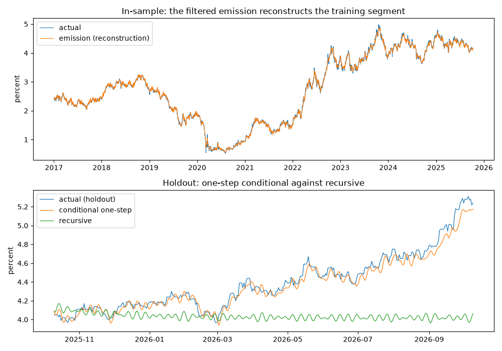
                       rmse     mae  mape_pct
one-step (log)       0.0140  0.0110    0.7365
one-step (level)     0.0639  0.0494    1.0965
recursive (level)    0.4873  0.3747    8.0936
random walk (level)  0.0352  0.0231    0.5218

The paths over the full sample, in training units

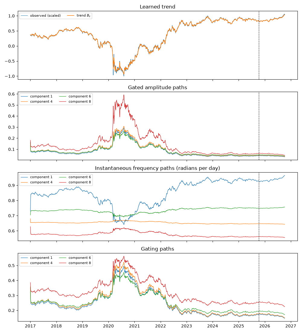
Figures 3 to 6. decompose(y, scaled=True) runs the trained network over training and holdout together and returns the paths in the scale the network trained on, which is how the paper draws them. Four of the eight components are shown, chosen by power share.

paths = res.decompose(y, scaled=True)
shown = np.argsort(res.power_share)[::-1][:4]
boundary = dates[split]

fig, axes = plt.subplots(4, 1, figsize=(10, 11), sharex=True)
axes[0].plot(dates, paths["observed"], lw=0.7, label="observed (scaled)")
axes[0].plot(dates, paths["trend"], lw=1.2, label="trend $B_t$")
axes[0].set_title("Learned trend")
for j in shown:
    axes[1].plot(dates, paths["amplitude"][:, j], lw=0.9, label=f"component {j + 1}")
    axes[2].plot(dates, paths["frequency"][:, j], lw=0.9, label=f"component {j + 1}")
    axes[3].plot(dates, paths["gate"][:, j], lw=0.9, label=f"component {j + 1}")
axes[1].set_title("Gated amplitude paths")
axes[2].set_title("Instantaneous frequency paths (radians per day)")
axes[3].set_title("Gating paths")
for ax in axes:
    ax.axvline(boundary, color="k", ls="--", lw=0.8)
    ax.legend(loc="upper left", fontsize=8, ncol=2)
plt.tight_layout()

The 2020 window in spectral-state coordinates

The paper reads frequency convergence with amplitude concentration around the 2020 shock. In the coordinates of the spectral state that is a joint contraction of the dispersion and the effective count, and the velocity says when the measure moved. The windows are the six months before March 2020 and the six months from it.

state = res.spectral_state()  # training-segment rows; the paths above cover the full sample
coords = state.to_pandas(index=dates[: state.nobs])

before = coords.loc["2019-09-01":"2020-02-29"]
after = coords.loc["2020-03-01":"2020-08-31"]
comparison = pd.DataFrame(
    {"before": before.mean(), "after": after.mean()},
).loc[["centroid", "dispersion", "effective_count", "participation_ratio", "velocity"]]
comparison["change"] = comparison["after"] - comparison["before"]
print(comparison.round(4).to_string())
print(f"disentanglement over the training segment: {state.disentanglement_score:.3f}")

fig, axes = plt.subplots(3, 1, figsize=(10, 8), sharex=True)
axes[0].plot(coords.index, coords["centroid"], lw=0.9, label="centroid")
axes[0].fill_between(
    coords.index,
    coords["centroid"] - coords["dispersion"],
    coords["centroid"] + coords["dispersion"],
    alpha=0.25,
    label="centroid $\\pm$ dispersion",
)
axes[0].set_ylabel("rad/day")
axes[1].plot(coords.index, coords["effective_count"], lw=0.9, label="effective count")
axes[1].plot(coords.index, coords["participation_ratio"], lw=0.9, label="participation ratio")
axes[1].set_ylabel("components")
axes[2].plot(coords.index, coords["velocity"], lw=0.7, label="velocity")
axes[2].plot(coords.index, coords["velocity_frequency"], lw=0.7, label="frequency part")
axes[2].plot(coords.index, coords["velocity_mass"], lw=0.7, label="mass part")
axes[2].set_ylabel("$W_1$ per day")
for ax in axes:
    ax.axvspan(
        pd.Timestamp("2020-03-01"), pd.Timestamp("2020-08-31"), color="0.85", label="2020 window"
    )
    ax.legend(loc="upper left", fontsize=8, ncol=2)
axes[0].set_title("Spectral state of the training segment, 2020 window shaded")
plt.tight_layout()

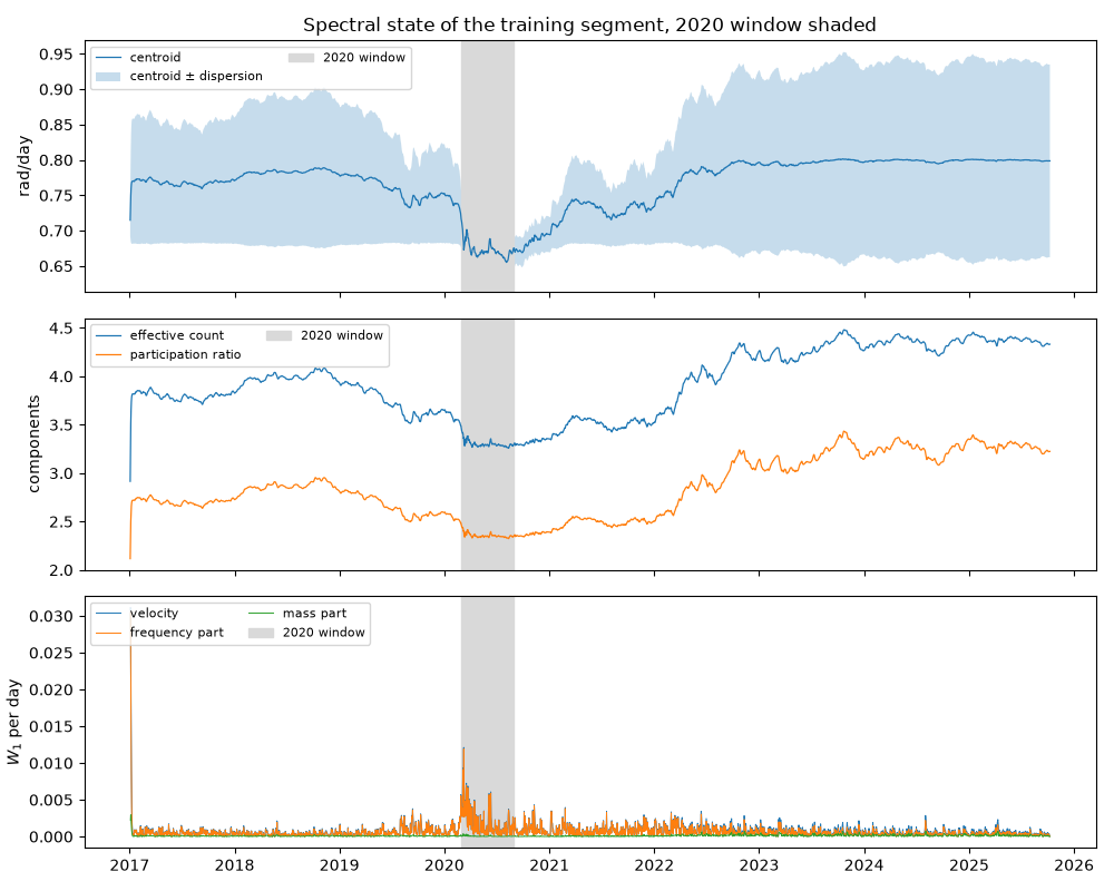
                     before   after  change
centroid             0.7446  0.6725 -0.0721
dispersion           0.0628  0.0219 -0.0409
effective_count      3.5965  3.3007 -0.2958
participation_ratio  2.5558  2.3550 -0.2008
velocity             0.0009  0.0018  0.0008
disentanglement over the training segment: 0.932

Reading it

A contraction in both dispersion and effective_count across the window is the compression reading; a fall in one without the other is a different story, and the disentanglement score says how far the per-component paths behind it can be trusted. Whatever this shortened fit shows, the claim rests on the published configuration and on its stability across seeds; the coordinates are permutation-invariant, so a seed sweep of the reproduction example is the natural test.