A series with a known decomposition

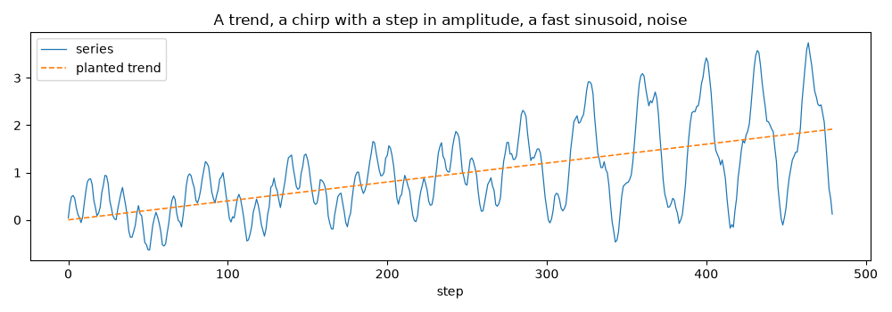
The model is handed a series built from the parts it is meant to find: a linear trend, a slow oscillation whose frequency rises through the sample and whose amplitude steps up two-thirds of the way through, a faster oscillation at a fixed frequency, and noise. The example fits the default filtered alignment, reads every path off the result, checks the identity that ties them together, and then asks the only question that matters about a decomposition with a known answer: how did the network divide the series between its trend head and its components?

The answer, on a short schedule, is the behaviour the user guide’s nuances page describes: the trend head reconstructs the series and the components carry little. The example is therefore less a demonstration that the model recovers planted sinusoids than a reading of what it does instead, with the tools that make that reading quick.

The series

Four hundred and eighty steps. The slow component’s frequency runs from 0.08 to 0.20 radians per step (periods of 79 down to 31 steps), its amplitude from 0.5 to 1.5 around step 300; the fast component sits at 0.60 (a period of about 10 steps).

import matplotlib.pyplot as plt
import numpy as np

from ns_sdn.spectral_decomposition import NSSDN, Stage

rng = np.random.default_rng(7)
n = 480
t = np.arange(n, dtype=float)
omega_slow = 0.08 + 0.00025 * t
amp_slow = 1.0 + 0.5 * np.tanh((t - 300) / 30)
slow = amp_slow * np.sin(np.cumsum(omega_slow))
fast = 0.4 * np.sin(0.60 * t)
trend_true = 0.004 * t
y = trend_true + slow + fast + 0.05 * rng.standard_normal(n)

fig, ax = plt.subplots(figsize=(10, 3.5))
ax.plot(t, y, lw=0.9, label="series")
ax.plot(t, trend_true, lw=1.2, ls="--", label="planted trend")
ax.set_xlabel("step")
ax.legend(loc="upper left")
ax.set_title("A trend, a chirp with a step in amplitude, a fast sinusoid, noise")
plt.tight_layout()

Fit

Three components, a 32-dimensional state and one stage of three hundred Adam steps: a fraction of the published configuration, chosen so the page builds in under a minute. seed fixes the initialization.

res = NSSDN(y, k=3, state_dim=32, schedule=(Stage(5e-3, 300),), seed=0).fit()
print(res.summary())

                                       NSSDN(k=3) Results
================================================================================================
Model:          NSSDN(k=3, d=32, gru, filtered)  Log-likelihood:                          49.883
Objective:                                  mse  AIC:                                   7554.234
Scaling:                                 minmax  BIC:                                  23519.332
Observations:                               479  HQIC:                                 13830.318
Parameters:                                3827  One-step RMSE:                          0.21804
Gating:                                    True  Emission RMSE:                        0.0177576
------------------------------------------------------------------------------------------------
                mean amp   mean freq   period   mean gate      mix   power share
component 1       0.0339      0.6218     10.1       0.102   +0.238         0.349
component 2       0.0228      0.7396      8.5       0.085   +0.320         0.358
component 3       0.0641      0.7694      8.2       0.132   -0.127         0.293
================================================================================================
Filtered alignment: the emission at t conditions on y[t], so emission is a reconstruction of the
observed series and fittedvalues report the emission at t as the one-step forecast of y[t+1]
(the published protocol); compare against a random walk before reading them as skill.
llf is a concentrated Gaussian likelihood at a penalized fit and n_params the nominal weight
count; criteria compare k within one configuration only.
Components are identified up to permutation; indices are not stable across refits.

The identity

Trend plus the sum of the component contributions is the emission, exactly, and the emission reconstructs the series closely: under the filtered alignment the state at t has seen y[t].

rebuilt = res.trend + res.components.sum(axis=1)
print("identity holds:", bool(np.allclose(rebuilt, res.emission, atol=1e-5)))
print(f"emission RMSE: {np.sqrt(np.mean(res.reconstruction_resid**2)):.4f}")
print(f"one-step RMSE: {np.sqrt(res.sigma2):.4f}")

identity holds: True
emission RMSE: 0.0178
one-step RMSE: 0.2180

Where the variance went

The question with a known answer. The planted oscillations account for most of the series’ variance; the decomposition’s oscillation is what the components account for.

parts = {
    "series": y,
    "planted oscillation": slow + fast,
    "fitted trend": res.trend,
    "fitted oscillation": res.oscillation,
}
for name, values in parts.items():
    print(f"{name:>22s} variance {np.var(values):8.4f}")

fig, axes = plt.subplots(2, 1, figsize=(10, 6), sharex=True)
axes[0].plot(t, y, lw=0.8, label="series")
axes[0].plot(t, res.emission, lw=0.8, label="emission")
axes[0].plot(t, res.trend, lw=1.4, label="trend head $B_t$")
axes[0].legend(loc="upper left")
axes[0].set_title("The trend head tracks the series; the emission is trend plus components")
axes[1].plot(t, slow + fast, lw=0.8, label="planted oscillation")
axes[1].plot(t, res.oscillation, lw=1.2, label="components' contribution")
axes[1].legend(loc="upper left")
axes[1].set_xlabel("step")
plt.tight_layout()

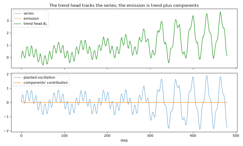
             series variance   0.8482
planted oscillation variance   0.5613
       fitted trend variance   0.8472
 fitted oscillation variance   0.0001

The component paths

Gated amplitude and instantaneous frequency per component, the paper’s Figures 4 and 5, with the planted frequencies drawn through the second panel. The frequencies are read in radians per step.

fig, axes = plt.subplots(3, 1, figsize=(10, 8), sharex=True)
for j in range(res.k):
    axes[0].plot(t, res.amplitude[:, j], label=f"component {j + 1}")
    axes[1].plot(t, res.frequency[:, j], label=f"component {j + 1}")
    axes[2].plot(t, res.gate[:, j], label=f"component {j + 1}")
axes[1].plot(t, omega_slow, color="k", ls="--", lw=1, label="planted slow")
axes[1].axhline(0.60, color="k", ls=":", lw=1, label="planted fast")
axes[0].set_ylabel("gated amplitude")
axes[1].set_ylabel("frequency (rad/step)")
axes[2].set_ylabel("gate")
axes[2].set_xlabel("step")
for ax in axes:
    ax.legend(loc="upper right", fontsize=8, ncol=2)
axes[0].set_title("Amplitude, frequency and gate paths against the planted frequencies")
plt.tight_layout()

print("mean frequency per component:", res.frequency.mean(axis=0).round(3))
print("power share per component:   ", res.power_share.round(3))

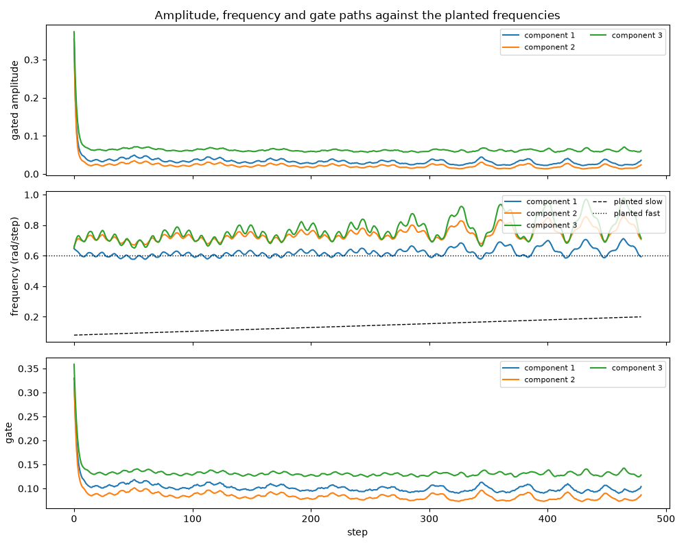
mean frequency per component: [0.622 0.74  0.769]
power share per component:    [0.349 0.358 0.293]

The spectral state

The same reading in permutation-invariant coordinates: the centroid and dispersion of the power-weighted frequency measure, and how many components it effectively uses.

state = res.spectral_state()
print(state.summary())

fig, axes = plt.subplots(2, 1, figsize=(10, 5), sharex=True)
axes[0].plot(t, state.centroid, label="centroid")
axes[0].fill_between(
    t,
    state.centroid - state.dispersion,
    state.centroid + state.dispersion,
    alpha=0.25,
    label="centroid $\\pm$ dispersion",
)
axes[0].set_ylabel("frequency (rad/step)")
axes[0].legend(loc="upper right")
axes[1].plot(t, state.effective_count, label="effective count")
axes[1].plot(t, state.participation_ratio, label="participation ratio")
axes[1].set_ylim(0.9, res.k + 0.1)
axes[1].set_ylabel("components")
axes[1].set_xlabel("step")
axes[1].legend(loc="upper right")
axes[0].set_title("Spectral-state coordinates over the sample")
plt.tight_layout()

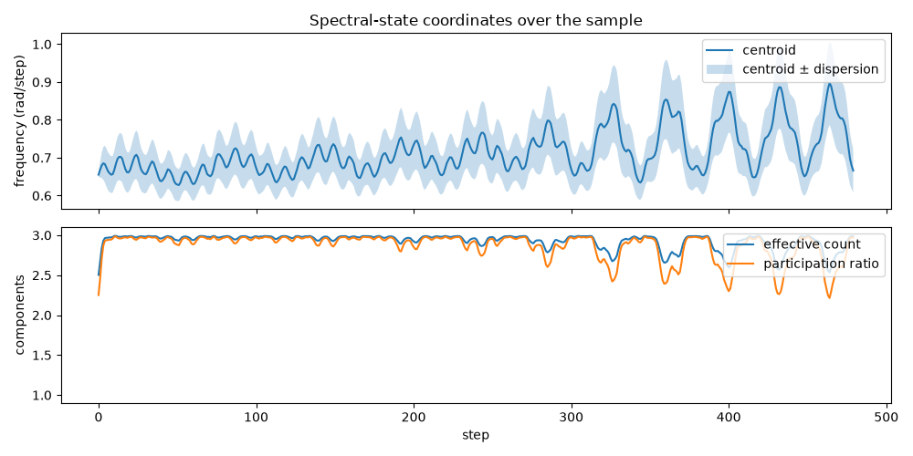
                              Spectral state (k=3)
================================================================================
Rows:                              480  Disentanglement:                 0.920
Active threshold:                 0.01  Mean active:                      3.00
--------------------------------------------------------------------------------
coordinate                             min / mean / max
centroid                       0.6278 / 0.7129 / 0.8973
dispersion                  0.006281 / 0.06649 / 0.1134
effective count                   2.503 / 2.926 / 2.991
participation ratio               2.214 / 2.863 / 2.982
velocity                   0.001278 / 0.01072 / 0.03347
velocity (frequency)     0.0007522 / 0.009353 / 0.02808
velocity (mass)          1.15e-05 / 0.001378 / 0.007032
================================================================================
Diagnostics of a model trained on the prediction criterion alone; nothing here
enters a loss.
Identifiability degrades as frequencies converge: compression is also the regime
of weakest disentanglement, and per-component readings of inactive rows are not
meaningful.

The predicted alignment

Trained to predict y[t] from the state after y[t - 1] instead, the network is a forecaster and the one-step error is the thing it minimizes. The random walk is the benchmark: it predicts each value by the one before it, which on a smooth series is already most of the way.

fwd = NSSDN(y, k=3, state_dim=32, alignment="predicted", schedule=(Stage(5e-3, 300),), seed=0).fit()
naive = y[:-1]
target = y[1:]
rmse = lambda a, b: float(np.sqrt(np.mean((a - b) ** 2)))  # noqa: E731
print(f"one-step RMSE, filtered:  {rmse(target, res.fittedvalues):.4f}")
print(f"one-step RMSE, predicted: {rmse(target, fwd.fittedvalues):.4f}")
print(f"one-step RMSE, random walk: {rmse(target, naive):.4f}")
print(f"predicted alignment, fitted oscillation variance: {np.var(fwd.oscillation):.4f}")

one-step RMSE, filtered:  0.2180
one-step RMSE, predicted: 0.0869
one-step RMSE, random walk: 0.2166
predicted alignment, fitted oscillation variance: 0.0003

What this shows

On this schedule the trend head has done the work under both alignments: it reconstructs the series under the filtered one and reproduces the previous value under the predicted one, while the components’ share of the variance stays near zero. One component’s frequency does settle close to the planted 0.60, which is also near the softplus initialization, but its gated amplitude is a few hundredths; nothing finds the 0.08-to-0.20 chirp, whose frequency the drift penalty would have to be pulled a long way to reach. The paths are smooth and the identities hold, which is what the package guarantees; whether the components carry the oscillation is a property of the fit, not of the API, and the tools above are how to check it. The published DGS10 run, with sixteen components and three thousand steps, is the configuration the papers read structure from; the next example runs a shorter version of it.