Equity volatility: GARCH, asymmetric GARCH and stochastic volatility

Daily equity returns have a conditional variance that clusters, responds more to falls than to rises, and is nearly integrated. The GARCH family models that variance as a deterministic function of past returns; the stochastic-volatility model gives it its own innovation and is estimated by quasi-maximum likelihood on the linearized model or by Markov chain Monte Carlo on the exact one.

This example fits GARCH(1,1), GJR-GARCH and EGARCH to NASDAQ Composite returns, tests the leverage effect, estimates a stochastic-volatility model both ways, and compares all of them as one-day value-at-risk forecasters with the Kupiec and Christoffersen coverage tests and the pinball loss.

Data

Daily closes of the NASDAQ Composite, 2008 to 2013, as percent log returns: six years that open with the 2008 crisis and contain the 2010 flash crash and the 2011 correction. The window is kept short because the stochastic-volatility sampler below is the costly step; extend end for a longer backtest.

import matplotlib.pyplot as plt
import numpy as np
from scipy import stats

from cultivars.forecast.scoring import pinball_loss
from cultivars.univariate.conditional_variance import EGARCH, GARCH, GJR
from cultivars.univariate.stochastic_volatility import SV

from _fred import fetch

prices = fetch({"nasdaq": "NASDAQCOM"}, start="2007-12-31", end="2013-12-31")
returns = (100.0 * np.log(prices["nasdaq"]).diff()).dropna()
r = returns.to_numpy()
print(f"{len(r)} trading days")
print(
    f"mean {r.mean():.3f}  sd {r.std():.3f}  skew {stats.skew(r):.2f}  "
    f"excess kurtosis {stats.kurtosis(r):.2f}"
)

1511 trading days
mean 0.030  sd 1.607  skew -0.22  excess kurtosis 6.09

The GARCH family

Three one-lag specifications with a constant mean. GJR adds an indicator for negative returns to the ARCH term; EGARCH models the log variance with a signed and an absolute innovation term. All three report persistence and its implied half-life in days.

garch = GARCH(r, p=1, q=1).fit()
gjr = GJR(r, p=1, o=1, q=1).fit()
egarch = EGARCH(r, p=1, o=1, q=1).fit()
print(garch.summary())
print(gjr.summary())
for label, result in (("GARCH", garch), ("GJR", gjr), ("EGARCH", egarch)):
    print(
        f"{label:7s}  persistence {result.persistence:.4f}  "
        f"half-life {result.half_life:6.1f} days  leverage: {result.has_leverage}"
    )

                              GARCH(1, 1) Results
================================================================================
Model:                     GARCH(1, 1)  Log-likelihood:              -2495.571
Mean:                         constant  AIC:                          4999.141
AR lags:                             0  BIC:                          5020.423
Observations:                     1511  HQIC:                         5007.067
--------------------------------------------------------------------------------
               coef
const        0.0973
omega        0.0262
alpha[1]     0.0987
beta[1]      0.8888
================================================================================
Persistence: 0.9875   Covariance stationary: True   Half-life: 55.0
Unconditional variance: 2.0908
Standard errors are not yet available for this estimator.
                              GJR(1, 1, 1) Results
================================================================================
Model:                    GJR(1, 1, 1)  Log-likelihood:              -2461.774
Mean:                         constant  AIC:                          4933.547
AR lags:                             0  BIC:                          4960.150
Observations:                     1511  HQIC:                         4943.454
--------------------------------------------------------------------------------
               coef
const        0.0504
omega        0.0330
alpha[1]     0.0000
gamma[1]     0.1763
beta[1]      0.8912
================================================================================
Persistence: 0.9794   Covariance stationary: True   Half-life: 33.3
Unconditional variance: 1.6047
Standard errors are not yet available for this estimator.
GARCH    persistence 0.9875  half-life   55.0 days  leverage: False
GJR      persistence 0.9794  half-life   33.3 days  leverage: True
EGARCH   persistence 0.9749  half-life   27.3 days  leverage: True

Testing the leverage effect

GARCH is nested in GJR by the restriction that the asymmetry term is zero, so the likelihood-ratio test is valid, and the information criteria rank all three.

print(garch.likelihood_ratio_test(gjr).summary())
print(garch.compare(gjr, egarch, criterion="bic"))

                             Likelihood-Ratio Test
================================================================================
Verdict at 5%:                  reject
--------------------------------------------------------------------------------
null                   statistic   df   p-value
nested restriction       67.5941    1    0.0000
================================================================================
                            Model comparison by BIC
================================================================================
Observations:                     1511  Models:                              3
--------------------------------------------------------------------------------
model                     llf   k        BIC     dBIC
EGARCH(1, 1, 1)     -2460.822   5   4958.247    0.000
GJR(1, 1, 1)        -2461.774   5   4960.150    1.903
GARCH(1, 1)         -2495.571   4   5020.423   62.177
================================================================================
Ranked best-first; the final column is the gap to the best model.

Stochastic volatility two ways

The QML estimate linearizes the squared returns and runs the Kalman filter; it is fast and consistent but not efficient. The Gibbs sampler draws the log-variance path and the parameters jointly, with Student-t errors to absorb the fat tails that the Gaussian GARCH fits push into the variance. The sampler is the costly step and runs with a modest number of draws here; the split-Rhat and bulk effective sample sizes of the parameters say whether that was enough, and in a real application several thousand draws across multiple chains would be the norm.

sv_qml = SV(r).fit(method="qml")
print(sv_qml.summary())
posterior = SV(r, dist="t").sample(method="gibbs", n_draws=400, n_burn=150, seed=9)
print(posterior.summary())
report = posterior.convergence(include=("mu", "phi", "sigma2", "nu"))
for name, rhat, ess in zip(report.names, report.rhat, report.ess_bulk, strict=True):
    print(f"{name:7s}  split-Rhat {rhat:.3f}  bulk ESS {ess:7.1f}")

                           SV[constant, qml] Results
================================================================================
Method:                            qml  Log-likelihood:              -3502.320
Observations:                     1511  AIC:                          7012.640
Half-life:                        58.8  BIC:                          7033.922
--------------------------------------------------------------------------------
            estimate
mean       0.0300513
mu            0.1735
phi           0.9883
sigma2     0.0252633
================================================================================
The likelihood is the quasi-likelihood of the Harvey-Ruiz-Shephard
linearization, exact for the linearized model and consistent for this one;
compare only against other QML fits.
                           SV[constant, t] Posterior
================================================================================
Sampler:                         gibbs  Draws kept:                        250
Observations:                     1511  Burn-in:                           150
nu acceptance:                   0.233  Thin:                                1
--------------------------------------------------------------------------------
              mean       sd        5%       95%
mean        0.1230   0.0248    0.0813    0.1592
mu          0.1447   0.5211   -0.4822    0.8449
phi         0.9892   0.0042    0.9825    0.9957
sigma2      0.0245   0.0055    0.0159    0.0338
nu         10.4546   2.7261    6.5848   14.3555
================================================================================
Kim-Shephard-Chib mixture Gibbs sampler: exact conditional on the seven-
component approximation to log chi-squared(1).
Student-t observation noise as a scale mixture; under Gibbs the degrees of
freedom move by a random-walk Metropolis step on log(nu - 2) whose acceptance
rate is reported.
mu       split-Rhat 1.000  bulk ESS   337.8
phi      split-Rhat 1.028  bulk ESS    86.4
sigma2   split-Rhat 1.242  bulk ESS     3.6
nu       split-Rhat 1.917  bulk ESS     1.4

Conditional volatility paths

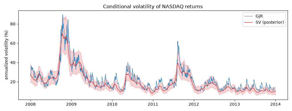
Annualized conditional volatility from GJR and from the posterior mean of the stochastic-volatility model, with the posterior 90 percent band. The stochastic-volatility path is smoother: it is an estimate of a latent state, not a function of the last return.

annualize = np.sqrt(252.0)
lower, upper = posterior.volatility_quantiles((0.05, 0.95))
fig, ax = plt.subplots(figsize=(10, 3.8))
ax.fill_between(returns.index, annualize * lower, annualize * upper, color="C3", alpha=0.2)
ax.plot(returns.index, annualize * gjr.conditional_volatility, color="C0", lw=0.8, label="GJR")
ax.plot(returns.index, annualize * posterior.volatility, color="C3", lw=1.0, label="SV (posterior)")
ax.set_ylabel("annualized volatility (%)")
ax.set_title("Conditional volatility of NASDAQ returns")
ax.legend()
fig.tight_layout()

Value-at-risk forecasts

The one-day 1 percent VaR is the quantile of the conditional distribution. For the GARCH models the conditional variance at date t is a function of returns through t - 1, so the in-sample path is a sequence of one-step-ahead forecasts conditional on the full-sample parameters; for the stochastic-volatility model the smoothed volatility uses the whole sample and is the more flattering object, which the comparison must say. Each VaR uses the quantile of its own error distribution: Gaussian for the GARCH fits, Student-t with the posterior-mean degrees of freedom for the sampler.

alpha = 0.01
z_gauss = stats.norm.ppf(alpha)
nu = posterior.params.nu
z_t = stats.t.ppf(alpha, nu) * np.sqrt((nu - 2.0) / nu) if nu is not None else z_gauss
value_at_risk = {
    "GARCH": garch.params["const"] + z_gauss * garch.conditional_volatility,
    "GJR": gjr.params["const"] + z_gauss * gjr.conditional_volatility,
    "EGARCH": egarch.params["const"] + z_gauss * egarch.conditional_volatility,
    "SV (QML)": sv_qml.mean + z_gauss * sv_qml.volatility,
    "SV (Gibbs)": posterior.params.mean + z_t * posterior.volatility,
}


def kupiec(hits: np.ndarray, level: float) -> tuple[float, float]:
    """Unconditional coverage likelihood-ratio test; returns the statistic and p-value."""
    n, x = hits.size, int(hits.sum())
    rate = x / n
    log_null = x * np.log(level) + (n - x) * np.log(1.0 - level)
    log_alt = x * np.log(rate) + (n - x) * np.log(1.0 - rate) if 0 < x < n else 0.0
    statistic = -2.0 * (log_null - log_alt)
    return float(statistic), float(stats.chi2.sf(statistic, 1))


def christoffersen(hits: np.ndarray) -> tuple[float, float]:
    """Independence likelihood-ratio test of first-order Markov clustering in the hits."""
    previous, current = hits[:-1], hits[1:]
    n00 = int(np.sum(~previous & ~current))
    n01 = int(np.sum(~previous & current))
    n10 = int(np.sum(previous & ~current))
    n11 = int(np.sum(previous & current))
    p01 = n01 / max(n00 + n01, 1)
    p11 = n11 / max(n10 + n11, 1)
    p = (n01 + n11) / max(n00 + n01 + n10 + n11, 1)

    def loglik(a: float, b: float) -> float:
        terms = (n00 * np.log1p(-a), n01 * np.log(a) if a > 0 else 0.0)
        terms += (n10 * np.log1p(-b), n11 * np.log(b) if b > 0 else 0.0)
        return float(sum(terms))

    statistic = -2.0 * (loglik(p, p) - loglik(p01, p11))
    return float(statistic), float(stats.chi2.sf(statistic, 1))


print(
    f"{'model':11s} {'hits':>5s} {'rate':>7s} {'Kupiec p':>9s} {'Christ. p':>10s} {'pinball':>9s}"
)
for label, var in value_at_risk.items():
    hits = r < var
    uc_stat, uc_p = kupiec(hits, alpha)
    ind_stat, ind_p = christoffersen(hits)
    loss = pinball_loss(r, var, alpha).mean()
    print(
        f"{label:11s} {int(hits.sum()):5d} {100 * hits.mean():6.2f}% {uc_p:9.3f} {ind_p:10.3f} "
        f"{loss:9.4f}"
    )

model        hits    rate  Kupiec p  Christ. p   pinball
GARCH          40   2.65%     0.000      0.140    0.0474
GJR            37   2.45%     0.000      0.173    0.0444
EGARCH         35   2.32%     0.000      0.197    0.0456
SV (QML)       38   2.51%     0.000      0.161    0.0422
SV (Gibbs)     23   1.52%     0.058      0.399    0.0360

Where the exceptions fall

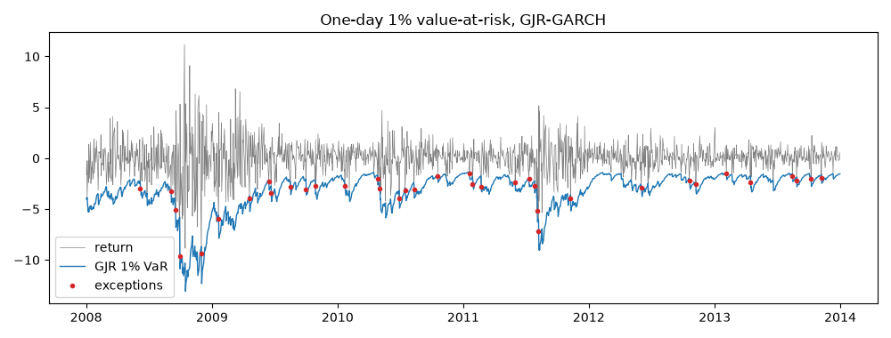
A model whose exceptions cluster in 2008 has the right unconditional rate for the wrong reason. The GJR exceptions are plotted against the returns and the VaR line.

fig, ax = plt.subplots(figsize=(10, 3.8))
ax.plot(returns.index, r, color="grey", lw=0.5, label="return")
ax.plot(returns.index, value_at_risk["GJR"], color="C0", lw=1.0, label="GJR 1% VaR")
exceptions = r < value_at_risk["GJR"]
ax.plot(returns.index[exceptions], r[exceptions], "o", color="C3", ms=3, label="exceptions")
ax.set_title("One-day 1% value-at-risk, GJR-GARCH")
ax.legend(loc="lower left")
fig.tight_layout()

What to take away

Asymmetry is the first thing the data ask for and the GJR term is usually several standard errors from zero on equity indices; the stochastic-volatility model fits the tails through its own innovation rather than through kurtosis in the variance. The VaR comparison here is in-sample and favours the smoothed stochastic-volatility path by construction; a rolling re-estimation with the Backtest harness is the out-of-sample version, and the coverage tests then apply to forecasts that were available when they were needed.