Monetary policy without recursiveness: heteroskedasticity and proxies

Recursive identification of a monetary policy shock rests on a timing assumption that nobody believes literally. Two alternatives drop it. Rigobon (2003) identifies from a shift in volatility: if the impact matrix is constant while the shock variances change across declared regimes, the regime covariances pin the impact matrix down with no zeros at all. Mertens and Ravn (2013) identify from an external instrument: a series correlated with the policy shock and with nothing else identifies the policy column by two-stage least squares on the reduced-form innovations.

The two combine naturally. The Volcker disinflation of 1979-82, when the Fed targeted reserves and let the funds rate move freely, is the canonical variance regime for a monetary shock, and the shock series it recovers in a small system can serve as the proxy in a larger one – the two-step design of Lanne and Lütkepohl (2008). This example runs that design and compares the three sets of impulse responses.

Data

Monthly 1965-2007: industrial production, the CPI, commodity prices, the funds rate and M2, in the units of the recursive example. The small system uses the first, second and fourth; the large system uses all five over the same sample and with the same lag order, so that the residual rows of the two VARs line up date for date.

import matplotlib.pyplot as plt
import numpy as np

from cultivars.multivariate.reduced_form.vector_autoregression import VAR
from cultivars.multivariate.structural.external_instruments import ProxySVAR
from cultivars.multivariate.structural.heteroskedacity import HeteroskedasticSVAR
from cultivars.multivariate.structural.zero_restrictions import RecursiveSVAR

from _fred import fetch

data = fetch(
    {"ip": "INDPRO", "cpi": "CPIAUCSL", "pcom": "PPIACO", "ffr": "FEDFUNDS", "m2": "M2SL"},
    start="1965-01-01",
    end="2007-12-01",
    units={"ip": "log", "cpi": "log", "pcom": "log", "m2": "log"},
)
data[["ip", "cpi", "pcom", "m2"]] *= 100.0
order = 12
small_names = ("ip", "cpi", "ffr")
small = VAR(data[list(small_names)].to_numpy(), order=order, names=small_names).fit()
dates = data.index[order:]

The variance regime

One label per residual row. The Volcker regime runs from October 1979, when the FOMC switched to non-borrowed-reserve targeting, to October 1982, when it abandoned it. Everything else is the calm regime; it is listed first, so the shocks are normalized to unit variance there and the reported ratios read as “how many times more volatile in 1979-82”.

volcker = (dates >= "1979-10-01") & (dates <= "1982-10-01")
regimes = np.where(volcker, "volcker", "calm")
print(f"{int(volcker.sum())} Volcker months, {int((~volcker).sum())} calm months")

37 Volcker months, 467 calm months

Identification through heteroskedasticity

With two regimes the rotation comes from an eigendecomposition and is unique when the variance ratios are distinct. The summary reports those ratios; the shock whose variance shifted most is in the first column. Nothing in the data labels it “monetary”, so the check is whether that shock’s impact pattern is the one a policy shock should have: it moves the funds rate on impact, by much more than it moves production or prices.

rigobon = HeteroskedasticSVAR(small, regimes, shock_names=("policy", "second", "third")).identify()
print(rigobon.summary())

horizon = 48
ffr = small_names.index("ffr")
policy = list(rigobon.shock_names).index("policy")
irf_rigobon = rigobon.irf(horizon)[:, :, policy]
irf_rigobon = irf_rigobon / irf_rigobon[0, ffr]

                                                       Structural VAR (heteroskedasticity)
==================================================================================================================================================
Scheme:                                               heteroskedasticity  Identified shocks:                                                3 of 3
Variables:                                                             3  Observations:                                                        504
Regimes:                                                               2  Variances in 'volcker' vs 'calm':                   21.019, 1.721, 1.176
Min ratio separation:                                             0.2002  Identification:                   WEAK: separation within sampling noise
--------------------------------------------------------------------------------------------------------------------------------------------------
impact of     policy    second     third
ip            0.0871    0.5838   -0.0770
cpi           0.0132    0.0315    0.1996
ffr           0.3017   -0.0014   -0.0303
==================================================================================================================================================
The impact matrix is assumed constant across the declared regimes ('calm', 'volcker'), with only the shock variances shifting; that assumption is
the entire identification. Shocks are unit-variance in the 'calm' regime, ordered by descending variance ratio, and labelled by their variance
behavior rather than by economics -- an economic name for any of them is a claim to be argued from outside the model. Near-equal ratios mean weak
identification; the separation is reported above.
Shocks are normalized to unit variance, so impact-column entries are responses to a one-standard-deviation structural shock.

The recursive benchmark

The same small system under the Cholesky ordering with the rate last, normalized the same way, is the comparison the literature always draws.

recursive = RecursiveSVAR(small, order=small_names).identify()
irf_recursive = recursive.irf(horizon)[:, :, ffr]
irf_recursive = irf_recursive / irf_recursive[0, ffr]

Correlation of the two shock series

If both schemes identify the same object the recovered shock series should be highly correlated. A low correlation means at least one of the identifying assumptions is wrong; it does not say which.

shock_rigobon = rigobon.structural_shocks()[:, policy]
shock_recursive = recursive.structural_shocks()[:, ffr]
correlation = np.corrcoef(shock_rigobon, shock_recursive)[0, 1]
print(f"Correlation of the two policy shock series: {correlation:.3f}")

Correlation of the two policy shock series: 0.971

Second step: the Rigobon shock as an external instrument

The shock recovered from the three-variable system is used as the proxy for the policy shock in a five-variable system that adds commodity prices and M2. The proxy is exogenous by construction with respect to the small system; its relevance in the large system is an empirical matter that the first-stage F statistic reports. The F statistic is the instrument’s whole claim to usefulness: below ten the identified column is unreliable (Montiel Olea, Stock and Watson 2021).

large_names = tuple(data.columns)
large = VAR(data.to_numpy(), order=order, names=large_names).fit()
proxy = ProxySVAR(large, shock_rigobon, shock="policy", normalize="ffr").identify()
print(proxy.summary())
ffr_large = large_names.index("ffr")
irf_proxy = proxy.irf(horizon)[:, :, list(proxy.shock_names).index("policy")]
irf_proxy = irf_proxy / irf_proxy[0, ffr_large]

                             Structural VAR (proxy)
================================================================================
Scheme:                          proxy  Identified shocks:              1 of 5
Variables:                           5  Observations:                      504
First-stage F:                 6698.44  Instruments:                         1
Normalization:       ffr > 0 on impact
--------------------------------------------------------------------------------
impact of      policy
ip             0.1473
cpi            0.0187
pcom           0.0326
ffr            0.4892
m2            -0.0350
================================================================================
External instrument: 1 proxy series assumed correlated with the 'policy' shock
and uncorrelated with every other structural shock. Relevance is reported below;
exogeneity is an assumption the instrument's construction must defend, because
no statistic here can.
Shocks are normalized to unit variance, so impact-column entries are responses
to a one-standard-deviation structural shock.
Only the listed shock columns are identified; the remaining structural shocks
exist but are not pinned down by these restrictions. Variance shares therefore
need not sum to one across the identified shocks, and the unidentified remainder
is exactly the variation the scheme is silent about.

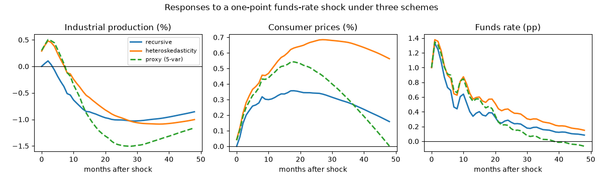
Three readings of the same shock

All three are normalized to a one-point impact increase in the funds rate. The recursive and heteroskedasticity responses come from the same three-variable system; the proxy responses come from the larger one, so differences there mix identification with specification.

labels = {"ip": "Industrial production (%)", "cpi": "Consumer prices (%)", "ffr": "Funds rate (pp)"}
steps = np.arange(horizon + 1)
fig, axes = plt.subplots(1, 3, figsize=(12, 3.6))
for ax, name in zip(axes, small_names, strict=True):
    ax.plot(steps, irf_recursive[:, small_names.index(name)], lw=2, label="recursive")
    ax.plot(steps, irf_rigobon[:, small_names.index(name)], lw=2, label="heteroskedasticity")
    ax.plot(steps, irf_proxy[:, large_names.index(name)], lw=2, ls="--", label="proxy (5-var)")
    ax.axhline(0.0, color="k", lw=0.8)
    ax.set_title(labels[name])
    ax.set_xlabel("months after shock")
axes[0].legend(fontsize=8)
fig.suptitle("Responses to a one-point funds-rate shock under three schemes")
fig.tight_layout()

What to take away

Heteroskedasticity identification is only as good as the regime declaration and the constant-impact assumption, and the variance ratios in the summary are its entire empirical content: ratios close to one for all but one shock mean the scheme identifies that shock well and the others barely at all. The proxy step inherits whatever mislabelling the first step made – a generated instrument is still an instrument, but its exogeneity is a claim about the small system, not a fact about the Fed. Where the three responses agree, the recursive timing assumption was not doing the work; where they diverge, it was.