Supply and demand shocks with long-run restrictions

Blanchard and Quah (1989) identify aggregate supply and demand shocks in a bivariate system of output growth and unemployment from one restriction at the infinite horizon: demand shocks have no permanent effect on the level of output. Nothing is assumed about impact timing, which is what makes the scheme a natural counterpart to the recursive one.

The restriction only makes sense if output is integrated of order one and unemployment is stationary, so the exercise begins with unit-root tests rather than with the VAR. It then applies the paper’s two pre-treatments – a break in mean growth in 1974 and a linear trend in unemployment – fits the system, identifies, and reads the cumulated responses and the variance shares.

Data

Real GDP (chained 2017 dollars) and the civilian unemployment rate, quarterly, 1948Q1 to 2019Q4. Growth is the continuously compounded quarterly percent change, units="cch" on FRED’s side, so the level of output is the cumulated sum of the series.

import matplotlib.pyplot as plt
import numpy as np

from cultivars.diagnostics.unit_roots import adf, kpss
from cultivars.multivariate.reduced_form.vector_autoregression import VAR
from cultivars.multivariate.structural.zero_restrictions import LongRunSVAR

from _fred import fetch

raw = fetch(
    {"gdp": "GDPC1", "u": "UNRATE"},
    start="1947-10-01",
    end="2019-12-01",
    frequency="q",
    aggregation_method="avg",
    units={"gdp": "cch"},
)
print(raw.tail())

                gdp    u
date
2018-10-01  0.14154  3.8
2019-01-01  0.62238  3.9
2019-04-01  0.83168  3.6
2019-07-01  1.16321  3.6
2019-10-01  0.67956  3.6

Integration orders

The long-run restriction needs output growth to be stationary (so the level has a unit root) and unemployment to be stationary in levels. ADF tests the unit-root null; KPSS tests the stationarity null. Reading them together is the standard check: a series that ADF rejects and KPSS does not is comfortably I(0).

for name, series, trend in (("gdp growth", raw["gdp"], "c"), ("unemployment", raw["u"], "c")):
    unit_root = adf(series.to_numpy(), trend=trend)
    stationary = kpss(series.to_numpy(), trend=trend)
    print(
        f"{name:14s}  ADF {unit_root.statistic:7.3f} (p={unit_root.pvalue:.3f}, "
        f"reject unit root: {unit_root.reject()})   KPSS {stationary.statistic:6.3f} "
        f"(reject stationarity: {stationary.reject()})"
    )

level = adf(np.cumsum(raw["gdp"].to_numpy()), trend="ct")
print(f"log GDP level   ADF {level.statistic:7.3f} (p={level.pvalue:.3f}) with trend")

gdp growth      ADF  -5.337 (p=0.000, reject unit root: True)   KPSS  0.449 (reject stationarity: False)
unemployment    ADF  -2.924 (p=0.043, reject unit root: True)   KPSS  0.558 (reject stationarity: True)
log GDP level   ADF  -1.046 (p=0.938) with trend

The paper’s pre-treatment

Blanchard and Quah demean growth separately before and after 1974Q1, where mean growth fell, and remove a linear trend from unemployment. Both adjustments are deterministic and leave the shocks untouched; they keep the VAR from spending its lags on a mean shift.

data = raw.copy()
post = data.index >= "1974-01-01"
data.loc[~post, "gdp"] -= data.loc[~post, "gdp"].mean()
data.loc[post, "gdp"] -= data.loc[post, "gdp"].mean()
t = np.arange(len(data), dtype=float)
coefficients = np.polyfit(t, data["u"].to_numpy(), 1)
data["u"] -= np.polyval(coefficients, t)
names = ("dy", "u")
endog = data.to_numpy()

Reduced form

The paper uses eight lags; the criteria below say how much of that the data support. The long-run factorization requires a stationary system, so the stability check is not optional here: a root near one would make the long-run multiplier matrix ill-conditioned.

selection = VAR(endog, order=1, names=names).lag_order_selection(max_lags=10)
print(selection.to_table())
var = VAR(endog, order=8, trend="n", names=names).fit()
stability = var.stability_check()
print(f"Largest companion root {stability.max_modulus:.3f}; stable: {stability.is_stable}")

                              Lag order selection
================================================================================
Observations:                      278  Maximum lags:                       10
Consensus:                        none
--------------------------------------------------------------------------------
p           AIC        BIC       HQIC       FPE
0        0.7015     0.7276     0.7120    2.0168
1       -3.2906    -3.2123    -3.2592    0.0372
2       -3.4751   -3.3446*   -3.4228*    0.0310
3      -3.4958*    -3.3131    -3.4225   0.0303*
4       -3.4723    -3.2374    -3.3781    0.0310
5       -3.4634    -3.1763    -3.3482    0.0313
6       -3.4805    -3.1412    -3.3444    0.0308
7       -3.4675    -3.0761    -3.3105    0.0312
8       -3.4644    -3.0208    -3.2864    0.0313
9       -3.4739    -2.9781    -3.2750    0.0310
10      -3.4909    -2.9429    -3.2711    0.0305
================================================================================
An asterisk marks each criterion's minimum. Every order was scored on the same
sample, so entries within a column are comparable; FPE is on a determinant
scale, so entries across columns are not.
Largest companion root 0.877; stable: True

Long-run identification

order=("dy", "u") declares output growth as the variable whose level only the first shock moves permanently. The first shock is therefore supply; the second, which has no long-run effect on output, is demand. The factorization normalizes both shocks to a positive long-run effect on their own variable, which for demand means a positive effect on unemployment; we flip that column so a demand shock is expansionary.

svar = LongRunSVAR(var, order=names).identify()
print(svar.summary())
print("Long-run impact (rows: dy, u; columns: supply, demand):")
print(svar.long_run_impact.round(3))

horizon = 40
irf = svar.irf(horizon)
cumulative = svar.irf(horizon, cumulative=True)
sign = np.ones(2)
if irf[0, 0, 1] < 0:
    sign[1] = -1.0
irf = irf * sign
cumulative = cumulative * sign

                           Structural VAR (long-run)
================================================================================
Scheme:                       long-run  Identified shocks:              2 of 2
Variables:                           2  Observations:                      280
--------------------------------------------------------------------------------
impact of         dy         u
dy            0.5701   -0.5584
u             0.0290    0.2675
================================================================================
Long-run triangularity in the ordering dy -> u: each shock has no permanent
effect on the variables before its position. The restriction binds cumulated
responses, so on differenced data it restricts levels.
Shocks are normalized to unit variance, so impact-column entries are responses
to a one-standard-deviation structural shock.
Long-run impact (rows: dy, u; columns: supply, demand):
[[ 0.769  0.   ]
 [-1.408  7.227]]

Cumulated responses

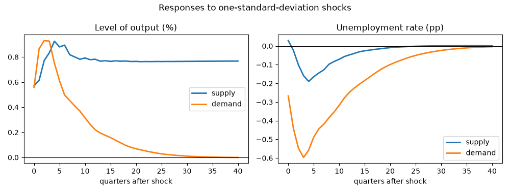
The output panel plots the cumulated response of growth, which is the response of the level. The demand response must return to zero; that is the restriction, not a finding. The supply response settles at the long-run impact. The unemployment panel is the response of the level directly.

fig, axes = plt.subplots(1, 2, figsize=(10, 3.8))
steps = np.arange(horizon + 1)
for j, shock in enumerate(("supply", "demand")):
    axes[0].plot(steps, cumulative[:, 0, j], lw=2, label=shock)
    axes[1].plot(steps, irf[:, 1, j], lw=2, label=shock)
axes[0].axhline(0.0, color="k", lw=0.8)
axes[1].axhline(0.0, color="k", lw=0.8)
axes[0].set_title("Level of output (%)")
axes[1].set_title("Unemployment rate (pp)")
for ax in axes:
    ax.set_xlabel("quarters after shock")
    ax.legend()
fig.suptitle("Responses to one-standard-deviation shocks")
fig.tight_layout()

Variance shares

Blanchard and Quah’s headline result is that demand shocks account for most of the forecast error variance of output at short horizons and a declining share as the horizon grows, by construction reaching zero in the level at infinity. For unemployment the demand share stays high.

fevd = svar.fevd(horizon)
print("Share of forecast error variance due to the demand shock")
for h in (1, 4, 8, 12, 24, 40):
    growth, unemployment = 100 * fevd[h, 0, 1], 100 * fevd[h, 1, 1]
    print(f"  h = {h:2d}   output growth {growth:5.1f}%   unemployment {unemployment:5.1f}%")

Share of forecast error variance due to the demand shock
  h =  1   output growth  55.4%   unemployment  99.5%
  h =  4   output growth  54.8%   unemployment  94.4%
  h =  8   output growth  56.2%   unemployment  93.1%
  h = 12   output growth  56.6%   unemployment  93.5%
  h = 24   output growth  56.7%   unemployment  93.9%
  h = 40   output growth  56.8%   unemployment  93.9%

Historical decomposition

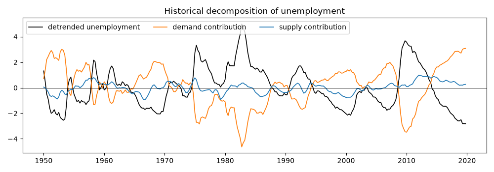
The decomposition attributes the deviation of unemployment from its deterministic path to the two shocks. The paper’s reading is that recessions are predominantly demand events, with the 1974-75 episode the one where supply plays a visible role.

decomposition = svar.historical_decomposition() * sign
dates = data.index[var.order :]
fig, ax = plt.subplots(figsize=(10, 3.5))
ax.plot(dates, data["u"].to_numpy()[var.order :], color="k", lw=1.2, label="detrended unemployment")
ax.plot(dates, decomposition[:, 1, 1], color="C1", lw=1.2, label="demand contribution")
ax.plot(dates, decomposition[:, 1, 0], color="C0", lw=1.2, label="supply contribution")
ax.axhline(0.0, color="k", lw=0.6)
ax.legend(loc="upper left", ncol=3)
ax.set_title("Historical decomposition of unemployment")
fig.tight_layout()

What to take away

Long-run restrictions buy identification without timing assumptions, at the price of estimating an infinite-horizon object from a finite sample: the long-run multiplier is a ratio of sums of VAR coefficients, and Faust and Leeper (1997) show how little the data say about it when the roots are large. The stability check and the size of the largest root are the first thing to report alongside any Blanchard-Quah result.